Can a physical robot play Atari 2600 games? PPO training within a Sim2Real framework enables Stretch 3 robot to overcome real-world delays, inertia, and noisy action transitions.
Introduction
The goal of this project was to determine whether it is possible to train a Reinforcement Learning (RL) policy in an environment that includes delay. RL is becoming increasingly popular, especially in robotics, yet as far as I know, no one has trained a policy that explicitly accounts for delay induced by robot dynamics. This matters because the model-free and general nature of RL could make it a powerful way to tackle more complex real-world robotic tasks.
What is Delayed Reinforcement Learning?
In the “vanilla” case, every action chosen by the policy is applied immediately, so the relationship between observation and action is straightforward.
On a physical system, however, this is no longer true. The robot has to physically move to execute an action, and that movement takes time because it is governed by real-world dynamics. This is very different from typical RL setups in video games, where all actions are instantaneous and purely virtual.
In this setting, the mapping from what the agent observes to the action that actually affects the environment becomes more complex, and that complexity needs to be built into the training environment to match real-world behavior as closely as possible and narrow the Sim2Real gap.
The Setup
The setup includes:
-
An Arcade Joystick (8BitDo’s Arcade Stick)
-
Hello Robot Stretch 3
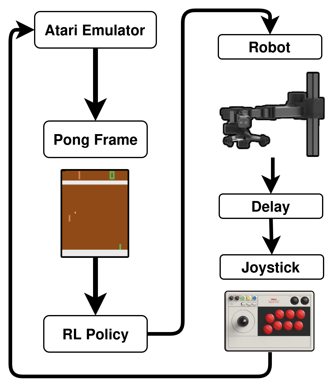
The full setup looks as follows:
Statistical Model The (Approach Taken)
The approach taken is stochastic. In real life, the robot takes time to move the joystick — it has inertia. The joystick has to move through transient states, so instead of a double-ended queue, the delay was modeled as a sequence of actions that are being piped into the environment.
For example, whenever the policy wants to go “up” and the joystick is in the “down” position, the environment is fed a sequence of actions: for some amount of time,
it repeats the current action (“down”) and then the neutral position (“no-op”) for another period of time. Not changing the state is not penalized. The timing was taken from real-life measurements.
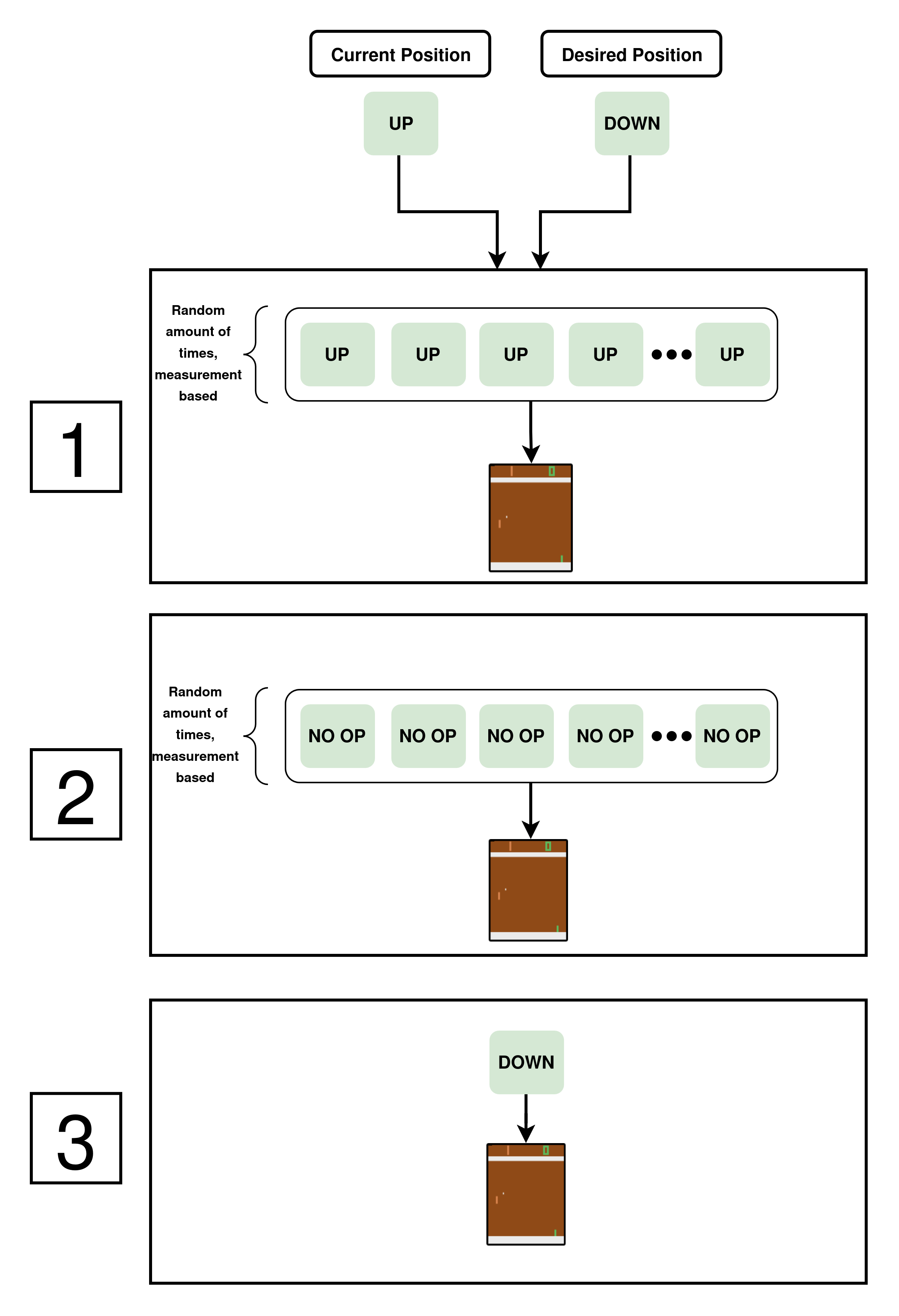
The movement from any state to the neutral one was measured and discretized: the delay measured was ~300 ms with a standard deviation of ~50 ms, so that was converted into 9 frames @ 30 FPS.
The challenge here was the discretization of the actions, as the joystick position and the game actions are discrete while the robot lives in the real world.
Delayed Action Queue (The “Wrong” Approach)
I refer to this approach as “wrong” because it is the one I have seen in the literature. When looking up “delayed reinforcement learning,” most work models the delay as an action buffer (a double-ended queue) of some fixed size: whenever the policy wants to take an action, that action is pushed into the queue and ultimately executed after the previous actions have been applied.
This does not represent physical robots for a simple reason: two opposing actions can still be taken one after the other, even with the queue. A simple example is the case in which a sequence of “UP” and “DOWN” actions is fed into the environment indefinitely. Given enough steps, the actions taken in such an environment would be “UP, DOWN, UP, DOWN, …” even though the queue exists.
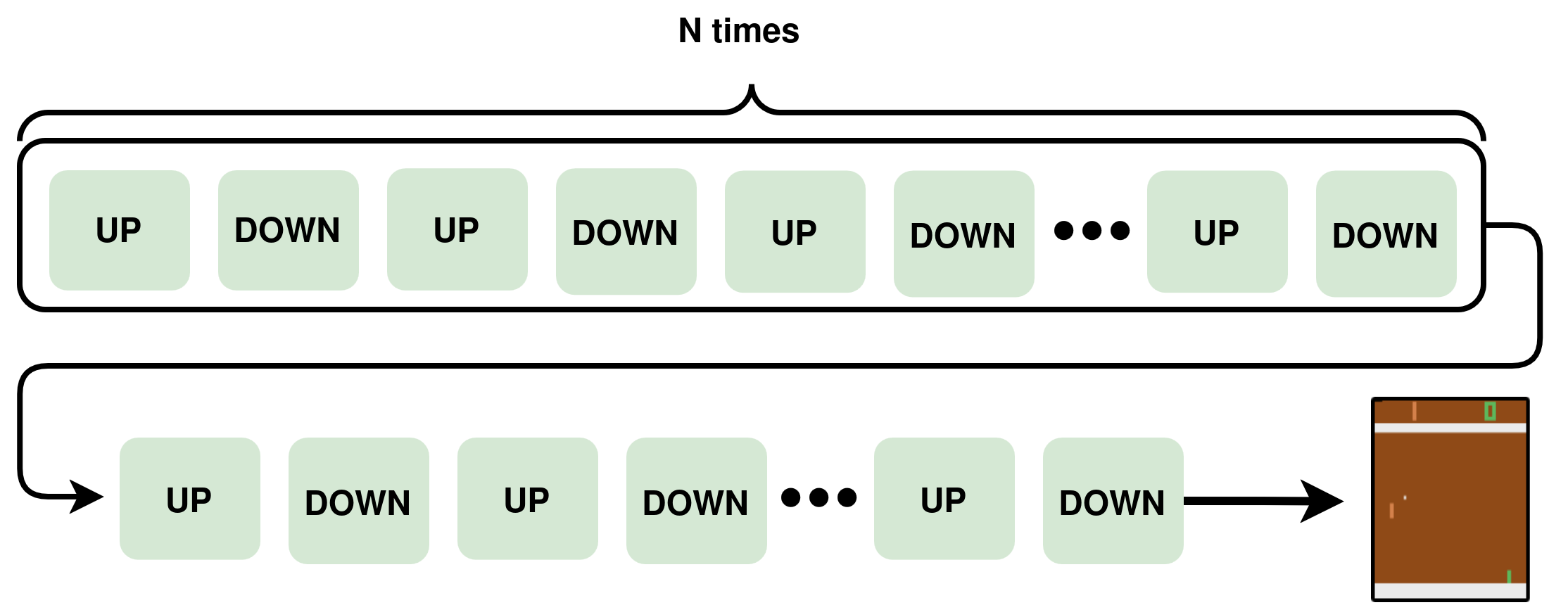
There would be a time difference between whenever the policy wanted to take these actions and when they are executed, but this setup still allows sharp changes in actions. That does not exist in real life, because the time between environment steps is very small (~33 ms @ 30 FPS), which is much smaller than the time that the robot takes to move the arcade stick in real life.
Comparison Between the Two Approaches
In the example above with the queue, the UP and DOWN actions alternate repeatedly, separated by a 1-second delay.
This is the same setting as before, but now with the transient states; it looks much more like real life.
To make this more concrete, each joystick transition is implemented as a short random sequence of phases.
For example:
| Phase |
Frames (example for one transition) |
Action applied to the game |
| Hold current state |
0–3 |
Current joystick action (e.g., DOWN) |
| Transition through neutral |
4–7 |
NO-OP (neutral position) |
| New state reached |
8+ |
Target joystick action (e.g., UP) |
Here, N_hold and N_total are derived from a sampled continuous delay, discretized into frames, so each transition has slightly different timing.
This is equivalent to a “sophisticated” frame-skip, where there is a sequence of actions being piped into the environment before the policy can choose the next action.
At first, the delay was considered to be constant — meaning that it always took the environment 9 frames for state transitions. This proved to be too easy: the policy would take
this behavior for granted, as it was completely consistent.
Domain Randomization
In the real robot, action delays are not constant, so using a single average delay would be misleading. Instead, I collected ~1,100 latency measurements over about one hour of robot motion and fit a Gaussian Mixture Model (GMM) to this data. Each Gaussian component has a very small standard deviation (around 3 ms), which is less than one frame at 30 FPS, so the mixture captures several tight “modes” of the delay distribution rather than a single broad average.
Because the simulator runs at 30 FPS, these continuous delay values are then mapped onto discrete frame counts. Concretely, when the policy requests a state change, the environment:
-
Samples a continuous delay (d) from the fitted GMM (with an extra small noise term so the policy cannot memorize an exact latency pattern).
-
Converts it to an integer number of frames: \(N = \operatorname{round}(d \cdot 30)\)
-
Uses the discretized delay as the effective latency: \(d_{\text{disc}} = \frac{N}{30}\).
-
Injects the action into the environment by holding or scheduling it over exactly \((N)\) frames.
In other words, the delay model lives in continuous time, but its samples are snapped to the 30 FPS grid before being applied, producing a realistic yet frame-aligned latency for the RL agent.
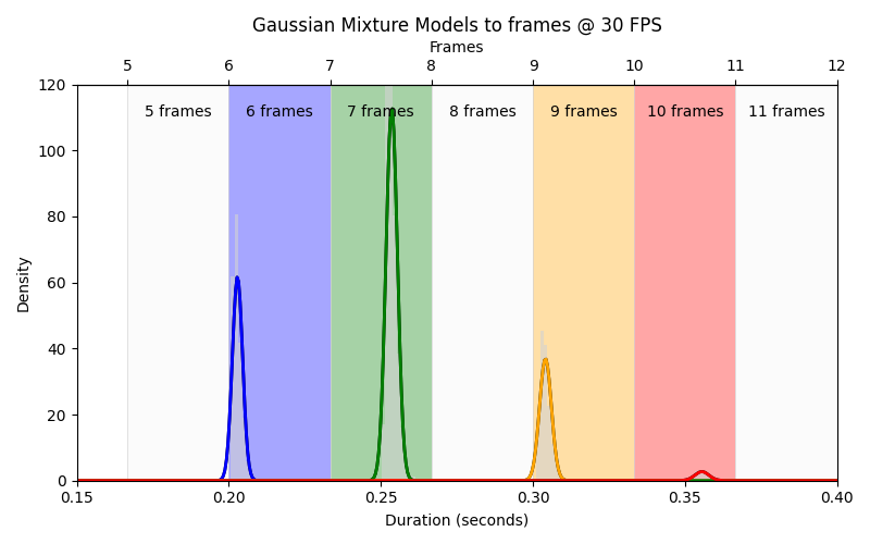
The figure above visualizes the mapping from continuous delay values to their corresponding integer frame counts at 30 FPS.
Training
Training PPO in the “vanilla” environment takes around 3M steps, using Stable-Baselines3’s default settings.
Training the policy under a constant delay value of around 15–20 environment steps takes a marginally longer time of around 50M steps.
In this case, PPO was not the best performing, and different algorithms were tested such as DQN, SAC, Recurrent PPO and Quantile Regression (QR)-DQN.
In this setup, Recurrent PPO (PPO based on LSTMs) and QR-DQN performed the best, but still took around 50M steps to train (~15× vs the vanilla case). However, as mentioned above, this did not incorporate any domain randomization and did not perform well on the real robot.
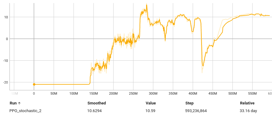
Finally, after introducing the stochastic delay model with domain randomization, PPO was the only algorithm that worked, while the rest (everything in Stable-Baselines3’s arsenal essentially) did not show meaningful improvement during training.
The training took significantly longer — around 500M steps. This is because the policy now cannot take anything about the timing for granted, and thus the whole task is less easily solvable.
Both the algorithm (PPO) and the emulator (Stella) run on the CPU, so this took a very long time in real life to train, because it did not benefit from GPUs at all.
A small summary of the approximate final episode rewards for the different setups is shown below:
| Environment setup |
Approx. final episode reward |
| Vanilla Pong (no delay) |
~20 |
| Constant delay (15–20 steps) |
~18 |
| GMM / randomized delay |
~14 |
Note the the max reward for Pong is 21 , and the reward represents the difference between the scores.
Results
The policy found a sweet spot, in which it did not need to move much (path of least resistance) in order to win the game — and essentially broke the game.
The full 40 min unedited footage (apart from a 10X speed increase) can be seen below.